Vertical Coordinate Reprojection: From Geoid to Ellipsoid

When doing surveys in the field, it’s critical to know the correct vertical elevation. But the earth has the shape of a lumpy potato, so it’s not easy to calculate the vertical elevation.

Traditionally the vertical elevation is calculated relative to a local system: the geoid. For the Netherlands the geoid ‘NAP height’ (https://www.rijkswaterstaat.nl/zakelijk/open-data/normaal-amsterdams-peil) is used – https://spatialreference.org/ref/epsg/5709/. The elevation is between minus 6.78 meter (Nieuwerkerk aan den IJssel) and 322.38 meter (Vaals).

For example the Dam square in Amsterdam has about 2.6 meter elevation:

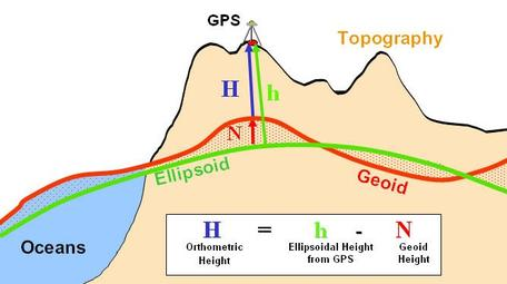
A more simple model (but less accurate) is to assume the earth has an ellipsoid shape. There is a difference between the ellipsoid and geoid, see:

With tool ‘Coordinates Converter’ (https://tools.propelleraero.com/coordinates-converter) we can transform coordinates between geoid and ellipsoid, for the Dam square in Amsterdam:

So for Amsterdam Dam square: 2.68 meter relative to the geoid (NAP) gives 45.6 meter relative to the ellipsoid.

From the command line we can use GDAL/PROJ tooling to convert from geoid to ellipsoid using tool ‘cs2cs’. In QGIS it’s installed in the bin directory (for example c:\Program Files\QGIS 3.32.0\bin).

For example convert from Dutch horizontal coordinates (EPSG:28992 ) + vertical coordinates (EPSG:5709 – according to the geoid model) to the ellipsoid model:

Here we use a Dutch composite coordinate systems EPSG:7415 = EPSG:28992 (horizontal) + EPSG:5709 (vertical). I’ve collected some composite EPSG codes for other countries at https://github.com/bertt/epsg

GDAL uses a set of TIF files to correctly transform the coordinates. IN QGIS they are installed in the ‘share/proj’ folder (for example c:\Program Files\QGIS 3.32.0\share\proj). For the Netherlands TIF file ‘nl_nsgi_naptrans2018.tif’ is used (download at https://cdn.proj.org/nl_nsgi_naptrans2018.tif). It looks like:

For the Netherlands it has values between 41 meter in Groningen and 47 meter in Limburg.

It can happen that the grids are not installed (to safe space). For example Docker image osgeo/gdal:ubuntu-small-3.6.3 does not have the grids (so we get 2.68 meter again when transforming):

When adding option ‘—only-best=yes’ there is a error message about the missing grid. When setting variable ‘PROJ_NETWORK=ON’ the grid is downloaded and the calculation goes well (result 45.663 meter).  We can also run tool ‘projsync’ (https://proj.org/en/9.2/apps/projsync.html) to download all the grids at once (670 MB).

More about this topic see:

– Convert between Orthometric and Ellipsoidal Elevations using GDAL https://spatialthoughts.com/2019/10/26/convert-between-orthometric-and-ellipsoidal-elevations-using-gdal/

– When Proj Grid-Shifts Disappear http://blog.cleverelephant.ca/2023/02/proj-network.html

Exploring 3D options of MapBox v3

At August 8 2023 there was a Mapbox announcement about supporting 3D environments in an upcoming release v3, see the blog post https://www.mapbox.com/blog/standard-core-style

There is a live demo site, see https://labs.mapbox.com/labs-standard/#16.64/48.86137/2.290976/-20/62. It shows 3D Tiles models (glTF/b3dm) like the Eiffel Tower in Paris and 3D model trees (glTF models):

Exploring at bit further, there are 2 new data sources defined: ‘model’ (for glTF 2.0 models) and ‘batched-model’ (for 3D Tiles – b3dm). With these new data sources we can add our own (building) 3D models and instanced 3D models (like trees, benches, traffic lights) to the map.

I’ve created some samples that demonstrate how to use these new data sources.

One sample is demonstrating how to add a 3D glTF model to the map using GeoJSON. In this demo a new building placed on the Dam Square in Amsterdam, see https://bertt.github.io/mapbox_3dtiles_samples/samples/standard/3dmodel/

The location of the building is defined in a GeoJSON file (building.geojson):

The glTF model (building.glb) is added in the ‘models’ section of style.json (see https://bertt.github.io/mapbox_3dtiles_samples/samples/standard/3dmodel/style.json)

In the building layer the building source and model are combined:

This construction works on a small number of items, but doesn’t scale well for a lot of items (like trees of a country). Instead of using a GeoJSON data source we can also use a vector tiles data source.

For a demo of using vector tiles in combination with a ‘model’ data source see trees of Utrecht demo (https://bertt.github.io/mapbox_3dtiles_samples/samples/standard/trees/#15.1/52.08999/5.12577/0/58).

In this case the location of the trees is defined in vector tiles (these are protocol buffer files), they are visualized using a tree.glb model:

Tree Layer:

The vector tiles are created by Tippecanoe, see https://bertt.wordpress.com/2023/01/06/creating-vector-pmtiles-with-tippecanoe/ for more information about this tool.

In a next blog I’ll explore  the new ‘batched-model’ data source for placing 3D models of buildings.

Overture Maps

Last week Overture Maps released a new world-wide dataset https://overturemaps.org/overture-maps-foundation-releases-first-world-wide-open-map-dataset/ (2023-07-26). The first release of this dataset was in April 2023 (https://overturemaps.org/download/overture-april-alpha-release-notes/).

Overture Maps is an effort of Amazon, Meta, Microsoft, TomTom and Esri, so big companies but notably missing are Apple and Google.

At https://overturemaps.org/download/ we can get more information about the data. There are 4 themes: Places, Buildings, Transportation and Administrative boundaries. The bulk of the data is processed OpenStreetMap data, but other sources can be added.

The data is available under licenses like CDLA Permissive v 2.0 and ODbL. The data is stored in Parquet files in Amazon S3 and Microsoft Azure, the schema of the data we can find at https://docs.overturemaps.org/

At https://github.com/OvertureMaps/data/blob/main/README.md#data-location the download urls are shown:

To browse/download the data on Azure we can use Microsoft Azure Storage Explorer, it looks like:

Poking around the data, we can see it’s quite big (totally 200 GB): places is 8 GB and buildings is 110 GB.

Let’s download the first buildings file:

It’s a bit of cryptic name that ‘20230725_211555_00082_tpd52_00e93efa-24f4-4014-b65a-38c7d2854ab4’ but it should be a Parquet file. So let’s start DuckDB on the command line and inspect it:

So in this file there are 8 million buildings, they have a geometry (WKB as blob) and some other attributes. After ‘D copy buildings to buildings.parquet’ we have a new file buildings.parquet (1.4 GB).

We can analyze the geometries with the DuckDB Spatial functions, for example get the centroids of the buildings:

The spatial functions are a subset of the PostGIS spatial functions, see for more information https://duckdb.org/docs/extensions/spatial.html 

But can we visualize this file in QGIS? Yes, but first we have to convert it to a GeoParquet (https://geoparquet.org/) file. A GeoParquet file is a regular Parquet file, but with some extra metadata about the geometries. See https://bertt.wordpress.com/2022/12/20/geoparquet-geospatial-vector-data-using-apache-parquet/ for more detailed information about GeoParquet.

Tool ‘gpq’ (https://github.com/planetlabs/gpq) can be used to convert from Parquet to GeoParquet.

Note: directly reading of the Overture Parquet files in gpq does not work yet, see https://github.com/planetlabs/gpq/issues/57

After drag and drop the file ‘buildings_geo.parquet’ to QGIS it looks like:

So the buildings are scattered around, the building parquet files are not spatially ordered. To get all the buildings in an area we have to download more building Parquet files.

In some cities the attributes height and numfloors are filled in, for example in Boston

So in these places we can make 3D Maps, like https://github.com/shi-works/Overture-Maps-Data-for-GIS

Some other nice sites with processed data:

– All the places in a map https://bdon.github.io/overture-tiles/places.html

– Buildings GeoParquet files per country https://beta.source.coop/cholmes/overture/browse/geoparquet-country

Do you know any other sites with processed data? Let us know in the comments!

Create 3D Terrain from LiDAR data

In modern 3D GIS viewers/game engines, a ‘terrain’ is used to model the real world 3D surface. In Cesium software the terrain consist of irregular triangles. Each triangle has a elevation attribute on the vertices. In places where the elevation changes a lot, more and smaller triangles are used.

The format used for the terrain is called ‘quantized-mesh’, for the specifications see https://github.com/CesiumGS/quantized-mesh. The quantized mesh is created on various levels (LOD’s), from level 0 (global level) to maximum level 20 (detailed level).

Creating such a terrain is not an easy task. There are challenges for handling large input datasets, long processing times and storing many (giga)bytes of data.

In this blog I’m going to describe a pipeline of tools that will simplify creating a quantized-mesh terrain. We’ll start with downloading raw LiDAR data (Points) for an area in The Netherlands. The raw data will be converted to GeoTIFF format (Image) and quantized-mesh format (mesh of triangles like a TIN) using Docker containers. We will visualize the terrain in browser client of Cesium (Cesium JS).

1] Downloading LiDAR data

There are many sources of LiDAR data, in this case we’ll start at https://www.geotiles.nl/ and download the LAZ file for area ‘69AZ2’ close to Maastricht:

$ wget https://ns_hwh.fundaments.nl/hwh-ahn/ahn4/01_LAZ/C_69AZ2.LAZ 

Its a 6GB file! So have some free diskspace for storing those 827.314.790 points.

2] Processing data

To process the LiDAR data we’ll use a pipeline in PDAL, see https://github.com/bertt/pietersberg/blob/main/pipeline.json

The pipeline reads the data, selects a small area (around Pietersberg), select points with classification=2 (ground points) and exports a GeoTIFF file with resolution 0.5m (dtm.tif – 272MB).

To run the pipeline in PDAL execute:

$ pdal pipeline pipeline.json

The resulting GeoTIFF looks like:

Now we run 2 commands in Docker to create the terrain tiles:

$ docker run –v $(pwd):/data -it geodan/terrainwarp 

and

$ docker run –v $(pwd):/data -it geodan/terraintiler 

The first command (terrainwarp) does the following:

– uses GDAL to fill in empty areas (using gdall_fillnodata);

– warp the image to global format EPSG:4326. It also converts the vertical projection to the ellipsoid (EPSG:4979).

– creates a VRT (Virtual Raster) of the processed images using gdalbuildvrt, the resulting file is to be used in the next step.

The second command (terraintiler) creates the quantized-mesh terrain tiles using the Cesium Terrain Builder tool (https://github.com/geo-data/cesium-terrain-builder) including the TileJSON file layer.json.

These tools have some more options, see https://github.com/geodan/terrain for more information.

3] Visualizing

Now we get a minimal Cesium client and start a webserver:

$ wget https://raw.githubusercontent.com/Geodan/terrain/main/samples/maastricht/index.html
$ python -m http.server 8000

Result should look like in a browser (port 8000):

Live demo: https://bertt.github.io/pietersberg/index.html . The same terrain can also be used in game engines like Unity3D and Unreal.

The terrain is normally used to visualize the hills and valleys. But it can also be used to visualize by elevation, slope or aspect (demo see https://geodan.github.io/terrain/samples/maastricht/index-elevation.html):

So in a few steps we can get from bulky LiDAR files to speedy 3D Terrain visualization in the browser or game engines. When processing multiple LAZ files there will be other challenges of course, but more about that in a follow up blog so stay tuned

Speed up data processing using GNU Parallel

GNU Parallel (https://www.gnu.org/software/parallel/) is a command-line utility designed to achieve parallel execution of tasks across multiple CPU cores. It promises  to speed up computationally intensive tasks on multi core machines.

https://www.amazon.com/GNU-Parallel-2018-Ole-Tange/dp/1387509888

To test this tool we’ll download a set of Digital Elevation Models (DEM) from Corsica (.ASC files) and process them in GDAL (reproject and convert to TIFF files).

First let’s download the DEM files from https://geoservices.ign.fr/rgealti (a 285MB zipped file):

$ wget --no-check-certificate https://wxs.ign.fr/9u5z4x13jqu05fb3o9cux5e1/telechargement/prepackage/RGEALTI-5M_PACK_CORSE_16-06-2021$RGEALTI_2-0_5M_ASC_LAMB93-IGN78C_D02A_2020-04-16/file/RGEALTI_2-0_5M_ASC_LAMB93-IGN78C_D02A_2020-04-16.7z

After unzip there are a lot of folders with long names, but somewhere there are 220 ASC files. Example filename is ‘RGEALTI_FXX_1155_6135_MNT_LAMB93_IGN78C.asc’. We can load them in QGIS (using projection EPSG:2154):

Now let’s process the 220 files with GNU Parallel:

$ time find *.asc | parallel --bar 'gdalwarp -s_srs EPSG:2154 -t_srs EPSG:4326 {} {=s:RGEALTI:warped:;s:asc:tif:=}'

Result of this process in a set of 220 GeoTIFFS in EPSG:4326.

A lot of things are happening in this single line command:

– Get a list of ASC files (find *.asc)

– On all the files do gdalwarp (from EPSG:2154 to EPSG:4326)

– Rename the output files, replace  prefix ‘RGEALTI’ with ‘warped’ and replace extension ‘asc’ to ‘tif’

The syntax ‘{=s:RGEALTI:warped:;s:asc:tif:=}’ for getting the output file names is a bit cryptic at first but it’s very powerful.

The process with Parallel took 1m32.028s on my machine for 220 ASC files.

But how long does it take when using only 1 CPU? For this we add ‘–j 1’ and run again:

$ time find *.asc | parallel –j 1 --bar 'gdalwarp -s_srs EPSG:2154 -t_srs EPSG:4326 {} {=s:RGEALTI:warped:;s:asc:tif:=}'

Now it takes 7m1.548s.

So about 4.5 times faster, this saves a lot of time! Imagine the time saving when running on very large datasets on a machine with many CPU’s…

The nice thing is we can apply GNU Parallel on any kind of data processing so this a huge time/money saver.

Getting started with photogrammetry

Photogrammetry is a technique used to create 3D models by analyzing photographs or images. It involves extracting information about the shape, size, and spatial relationships of objects from multiple images taken from different angles.

COLMAP is a popular open-source photogrammetry software that is widely used for 3D reconstruction and image-based modeling. It provides a comprehensive set of tools and algorithms for processing images and generating accurate 3D models.

In this blog we will download a set of images of a building and process them in COLMAP to create a 3D model.

At https://github.com/colmap/colmap/releases there are binaries (for Windows), I’ve used COLMAP-3.8-windows-cuda.zip. After unzip there is a colmap.bat file, click it to open the tool:

Now we need a set of images to process.

At https://onedrive.live.com/?authkey=%21AAQumsDDwZBIW3w&id=C58A258D760E1B58%2146879&cid=C58A258D760E1B58 there are 4 sample sets.

Or as alternative option you can take a camera and create a set of images.

For now we’ll download the smallest file (south-building.zip – 400MB). It contains 128 overlapping images of a building, for example:

In COLMAP we open menu Reconstruction –> Automatic Reconstruction and specify the ‘Workspace folder’ (to output files) and Image folder (for the input images). To speed up the process I’ll set Quality to Low and press Run…

The process takes a few minutes. When finished there is a 3D view with all the calculated camera positions and orientations of the input images, really impressive!

In the output folder there is a file ‘dense\0\meshed-poisson.ply’, we can drag and drop it in MeshLab (https://www.meshlab.net/) tool for further processing.

I’ve used a decimation tool to reduce the size a bit.

The final model is uploaded to Sketchfab see https://sketchfab.com/3d-models/south-building-013bf89103b44fda9650200400918dda

Conclusion: With COLMAP we can create a 3D model from a set of images using photogrammetry techniques in a few minutes. 

Adding objects to Google Photorealistic 3D Tiles

Last month Google released a set of Photorealistic 3D Tiles, it looks like:

Under the hood, it’s all just 3D Tiles in a Cesium viewer. So we should be able to add our own models/ 3D tilesets.

Let’s try to add a glTF model of a house (https://github.com/bertt/googlemaps3d/blob/main/3dtiles/building.glb), we want to have it right on the Dam square in Amsterdam (coordinates 4.892419,52.373158).

This is an easy task isn’t it?

Let’s first look up the altitude of the Dam square at https://www.ahn.nl/ahn-viewer, it’s 2.12 meter

Now we can add little code to the Cesium viewer to add the building:

var modelMatrix = Cesium.Transforms.eastNorthUpToFixedFrame(Cesium.Cartesian3.fromDegrees(4.892419,52.373158, 2.12));
var model = viewer.scene.primitives.add(Cesium.Model.fromGltf({
    url : 'building.glb',
    modelMatrix : modelMatrix,
}));

If we look at the result https://bertt.github.io/googlemaps3d/3dtiles/index_0.html we see a lot of things, but the building is missing…

Actually, the building is there but its hidden under the surface!

What’s happening?

Well it turns out the altitude we used (2.12 m) is relative to the local geoid model of the earth, but in case of Google Photorealistic 3D Tiles we need an altitude relative to the ellipsoid (see figure).

In the Netherlands the difference between the Geoid and Ellipsoid can be somewhere between 40 and 47 meter:

How can we convert from geoid to ellipsoid?

We’ll use GDAL command line tool ‘cs2cs’:

$ echo 121297.4362 487369.0122 2.12 |   cs2cs EPSG:7415 EPSG:4326+4979 -d 10
52.3731610577   4.8923002210 45.1026281869

Here we convert the coordinate from EPSG:7415 (this is a compound CRS, horizontal Dutch EPSG:28992, vertical EPSG:5709 – NAP) to EPSG:4326 (horizontal) and EPSG:4979 (vertical relative to the ellipsoid).

The resulting altitude (relative to the ellipsoid) is 45.1 meter.

Now the building is correctly placed, result see https://bertt.github.io/googlemaps3d/3dtiles/index_45.html

Create 3D Tiles from French LIDAR Data

By 2026, a national project aims to map the entire French territory in three dimensions. The National Institute of Geographic and Forestry Information (IGN) is behind this “project”, entitled “Lidar HD”, whose objective is to obtain a very precise 3D description of the territory.

The 3D Map will meet the needs of observation and analysis in many fields:

• Prevention of natural risks.
• Knowledge of the forestry resource.
• Monitoring of the common agricultural policy.
• Energy transition and sustainable urban development.
• Regional planning.
• Internal security.
• Revealing archaeological remains.

The project started in 2021 and should be finished in 2026. It will take 7000 hours of flying to cover the entire territory. At the moment, the Southern part of France is available for download:

In this blog we will download LIDAR data from Nimes (around the Arena), process the data in PDAL and visualize in Cesium 3D Tiles. The result you can already observe here https://bertt.github.io/nimes/

Download

On https://geoservices.ign.fr/lidarhd the Lidar data can be obtained from a map:

For Nimes there is file LIDARHD_1-0_LAZ_NP-0808_6305-2021.7z (405MB).

After downloading and unzip there are 4 LAZ files: Semis_2021_0808_6304_LA93_IGN69.laz (93MB),  Semis_2021_0808_6305_LA93_IGN69.laz (107MB), Semis_2021_0809_6304_LA93_IGN69.laz (98MB) and Semis_2021_0809_6305_LA93_IGN69.laz (96MB).

Using PDAL we can get some statistics:

$ pdal info Semis_2021_0808_6304_LA93_IGN69.laz --all

A lot of statistics are shown, like area (1121100), count (19148173),  creation_year (2021).

Data processing

We will use PDAL to merge the 4 files (filters.merge), select the area around the arena (filters.crop), classify the lidar points based on z value and write the result.

The processing pipeline looks like:

For the code of the pipeline see https://github.com/bertt/nimes/blob/main/pipeline.json

We can run the pipeline using:

$ pdal pipeline pipeline.json

Result is a file result.las (32MB). We load this file in CloudCompare (https://www.danielgm.net/cc/):

The next step is to create 3D Tiles (https://www.ogc.org/standard/3dtiles/) to visualize the Lidar data on the web. We’ll use tool ‘Go Cesium Point Cloud Tiler’ (https://github.com/mfbonfigli/gocesiumtiler).

$ gocesiumtiler -srid 2154 -input result.las -output 3dtiles -zoffset 60

As ‘srid’ we use 2154 (https://epsg.io/2154) the France coordinate system. As ‘zoffset’ we use 60 meter, to be able to show the terrain and the LIDAR data together.

A ‘3dtiles’ folder will be created containing a lot of files. The LIDAR data is in the pnts files, specs see https://github.com/CesiumGS/3d-tiles/tree/main/specification/TileFormats/PointCloud. The spatial placement of the tiles is defined in the tileset.json files, an octree tiling scheme is used.

Visualize in Cesium

As a last step we can add the 3D Tileset in Cesium, code see https://github.com/bertt/nimes/blob/main/index.html. Here we define the various colors for classified points based on z values.

Result

Result: see https://bertt.github.io/nimes/

Conclusion

In this blog we were able to download raw laseraltimetry data from France and create 3D Pointcloud Tiles.

It was a bit surprising to see that the download zip files contains multiple LAZ files, but we could merge those files using PDAL.

Another issue was the field ‘Classification’ was not used (at least in these files), maybe here classification like road, water, building can be added.

As next steps we can analyze the LIDAR data more, for example by detecting/extracting objects… But that’s for another blog…

So far the first French LIDAR downloads look quite promising

Geofabrik Vector Tiles

2023-08-01: Updating to MapLibre 3 and styles are renamed

One of our favorite sites to get OpenStreetMap data is https://download.geofabrik.de/, it offers OpenstreetMap data in various formats like raw data, shapefiles,
and pre-packaged tiles.

Last week there was an announcement (https://blog.geofabrik.de/?p=589) that the data is also available as vector tiles (experimental).

Let’s see how this works and download some vector tiles from Andorra (https://download.geofabrik.de/europe/andorra.html):

We can download a 3.5 MB zipped file containing vector tiles (*.pbf), levels ranging from level 0 to 14 and unzip to the ‘tiles’ directory:

$ wget http://download.geofabrik.de/europe/andorra-shortbread-1.0.tar.gz
$ mkdir tiles
$ tar -xvf andorra-shortbread-1.0.tar.gz –C tiles

We can drag and drop the pbf files to QGIS to inspect:

So the vector tiles contains things like OpenstreetMap boundaries, buildings, POI’s, streets and water polygons/lines.

Now we need a style to render nice maps.

The Versatiles project offers 3 styles – Colorful, Eclipse, Neutrino (https://github.com/versatiles-org/versatiles-styles)

$ wget https://github.com/versatiles-org/versatiles-styles/releases/latest/download/styles.tar.gz
$ mkdir styles
$ tar -xvf styles.tar.gz –C styles

After unpack of styles.tar.gz in the style directory there are 7 JSON files:

Let’s open eclipse.json, for “tiles” there is a reference to https://tiles.versatiles.org:

Change it so it points to our own webserver (where our vector tiles are hosted), for example:

And we need a basic MapLibre (https://maplibre.org/) html client that zooms in to Andorra  (https://github.com/bertt/geofabrik/blob/main/mvt/index_eclipse.html):

$ wget https://raw.githubusercontent.com/bertt/geofabrik/main/mvt/index_eclipse.html

Directory should look like: https://github.com/bertt/geofabrik/tree/main/mvt

Now start a local webserver and browse to index_eclipse.html

When testing we are encountering a strange error: Unimplemented Type 3:

The reason for this the tiles are gzip compressed, so either we must change the server zip settings or unzip the files (for example with script https://github.com/bertt/geofabrik/blob/main/mvt/unzip.sh). Run this script in the tiles directory.

After unzipping the maps should be working

Eclipse is very dark style (as the name implies) https://bertt.github.io/geofabrik/mvt/index_eclipse.html

Neutrino https://bertt.github.io/geofabrik/mvt/index_neutrino.html

Colorful https://bertt.github.io/geofabrik/mvt/index_colorful.html

The nice thing is we change that style of the maps easily by changing the style json files.

Create Vector Tiles from OpenStreetMap using Planetiler

OpenStreetMap (https://www.openstreetmap.org) is a free, editable map of the whole world that is being built by volunteers largely from scratch.When browsing the map we see classic raster tiles displayed (png format). Can we also create vector tiles from the OpenStreetMap and customize the style?

Of course we can!

Some steps we have to take:

– Download OpenStreetMap data;

– Create vector tiles;

– Style the vector tiles;

– Deploy the result.

Download data

The daily fresh raw OpenStreetMap data can be obtained at the great site http://download.geofabrik.de/ . There are download extracts available per region:

I want to create a map of the Netherlands, the data (1.1 GB) is available at http://download.geofabrik.de/europe/netherlands.html

In the next step we’ll use a tool that does the downloading automatically, we only need the name of the dataset for now (‘netherlands’). Adjust to your use case as needed.

Create vector tiles

There is an Open Source project that creates vector tiles from OpenStreetMap data: Planetiler https://github.com/onthegomap/planetiler

The most easy way is to run it in Docker:

$ docker run -e JAVA_TOOL_OPTIONS="-Xmx1g" -v "$(pwd)/data":/data ghcr.io/onthegomap/planetiler:latest --download --area=netherlands \
  --water-polygons-url=https://github.com/onthegomap/planetiler/raw/main/planetiler-core/src/test/resources/water-polygons-split-3857.zip \
  --natural-earth-url=https://github.com/onthegomap/planetiler/raw/main/planetiler-core/src/test/resources/natural_earth_vector.sqlite.zip

Note the area parameter used in this command: –area=netherlands

After some waiting a 700 MB MBTile file is created: output.mbtiles.

We can drag and drop it in QGIS:

Some random styling is applied here. Good coincidence it took an orange color for the Netherlands

Next we can convert the MBTile to PMTiles (https://protomaps.com/docs/pmtiles) for easy hosting:

$ pmtiles convert output.mbtiles netherlands.pmtiles

Result is a 683MB PMTile file.

Note: In a future version of Planetiler we can export to PMTiles directly, so the conversion step from MBTiles to PMTiles can be skipped.

Deployment

I’ve uploaded the file to Azure blob store, now can use ‘PMTiles Viewer’ to inspect:

https://protomaps.github.io/PMTiles/?url=https://flatgeobuf.blob.core.windows.net/fgb/netherlands.pmtiles

In the Metadata tab of the PMTiles Viewer we can see the map layers used:

We can see levels 0-14 are used in the file, when zooming in there’s lot’s of detailed information:

See https://openmaptiles.org/schema/ for the definition of the layers and fields used.

Styling

A basic Leaflet client is available at https://flatgeobuf.blob.core.windows.net/fgb/netherlands.html

The map style is defined in the Leaflet code:

         let paint_rules = [
            {
                dataLayer:"aeroway",
                symbolizer:new protomaps.PolygonSymbolizer({fill:"#ffffff"}),
              },
            {
                dataLayer:"landcover",
                symbolizer:new protomaps.PolygonSymbolizer({fill:"#819A20"}),
              },
            {
                dataLayer:"building",
                symbolizer:new protomaps.PolygonSymbolizer({fill:"#f2eae2"}),
              },
              {
                dataLayer:"water",
                symbolizer:new protomaps.PolygonSymbolizer({fill:"#80bde3"}),
              },
              {
                dataLayer:"park",
                symbolizer:new protomaps.PolygonSymbolizer({fill:"#819A20"}),
                filter: (z, f) => {
                  return f.props.class == "national_park";
                }
              },
                {
                dataLayer:"transportation",
                symbolizer:new protomaps.LineSymbolizer({color:"#bbb"}),
                filter: (z, f) => {
                  return f.props.class == "rail";
                }
                },
                {
                dataLayer:"transportation",
                symbolizer:new protomaps.LineSymbolizer({color:"#d1c1be"}),
                filter: (z, f) => {
                  return f.props.class == "tertiary" || f.props.class == "secondary" || f.props.class == "primary";
                }
                },
                {
                dataLayer:"boundary",
                symbolizer:new protomaps.LineSymbolizer({color:"#d1c1be"}),
              }
            ]

The style can be completely adjusted to your own needs. See the documentation https://protomaps.com/docs/frontends/leaflet#my-first-symbolizer for more styling options.

Conclusion

Using Planetiler and PMTiles we can easily create our own vector tiles from current OpenStreetMap data. The data we get from http://download.geofabrik.de/. Styling of the vector tiles can be done using the PMTiles symbology. PMTiles is designed for simple CDN deployment. So after copying the PMTile file and Leaflet HTML file to a blob storage our map is up and running. It doesn’t get more easy .